DSA Time Complexity
Runtime
To fully understand algorithms we must understand how to evaluate the time an algorithm needs to do its job, the runtime.
Exploring the runtime of algorithms is important because using an inefficient algorithm could make our program slow or even unworkable.
By understanding algorithm runtime we can choose the right algorithm for our need, and we can make our programs run faster and handle larger amounts of data effectively.
Actual Runtime
When considering the runtime for different algorithms, we will not look at the actual time an implemented algorithm uses to run, and here is why.
If we implement an algorithm in a programming language, and run that program, the actual time it will use depends on many factors:
- the programming language used to implement the algorithm
- how the programmer writes the program for the algorithm
- the compiler or interpreter used so that the implemented algorithm can run
- the hardware on the computer the algorithm is running on
- the operating system and other tasks going on on the computer
- the amount of data the algorithm is working on
With all these different factors playing a part in the actual runtime for an algorithm, how can we know if one algorithm is faster than another? We need to find a better measure of runtime.
Time Complexity
To evaluate and compare different algorithms, instead of looking at the actual runtime for an algorithm, it makes more sense to use something called time complexity.
Time complexity is more abstract than actual runtime, and does not consider factors such as programming language or hardware.
Time complexity is the number of operations needed to run an algorithm on large amounts of data. And the number of operations can be considered as time because the computer uses some time for each operation.
For example, in the algorithm that finds the lowest value in an array, each value in the array must be compared one time. Every such comparison can be considered an operation, and each operation takes a certain amount of time. So the total time the algorithm needs to find the lowest value depends on the number of values in the array.
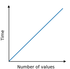
The time it takes to find the lowest value is therefore linear with the number of values. 100 values results in 100 comparisons, and 5000 values results in 5000 comparisons.
The relationship between time and the number of values in the array is linear, and can be displayed in a graph like this:
"One Operation"
When talking about "operations" here, "one operation" might take one or several CPU cycles, and it really is just a word helping us to abstract, so that we can understand what time complexity is, and so that we can find the time complexity for different algorithms.
One operation in an algorithm can be understood as something we do in each iteration of the algorithm, or for each piece of data, that takes constant time.
For example: Comparing two array elements, and swapping them if one is bigger than the other, like the Bubble sort algorithm does, can be understood as one operation. Understanding this as one, two, or three operations actually does not affect the time complexity for Bubble sort, because it takes constant time.
We say that an operation takes "constant time" if it takes the same time regardless of the amount of data (\(n\)) the algorithm is processing. Comparing two specific array elements, and swapping them if one is bigger than the other, takes the same time if the array contains 10 or 1000 elements.
Big O Notation
In mathematics, Big O notation is used to describe the upper bound of a function.
In computer science, Big O notation is used more specifically to find the worst case time complexity for an algorithm.
Big O notation uses a capital letter O with parenthesis \(O() \), and inside the parenthesis there is an expression that indicates the algorithm runtime. Runtime is usually expressed using \(n \), which is the number of values in the data set the algorithm is working on.
Below are some examples of Big O notation for different algorithms, just to get the idea:
| Time Complexity | Algorithm |
|---|---|
| \[ O(1) \] |
Looking up a specific element in an array, like this for example:
|
| \[ O(n) \] | Finding the lowest value. The algorithm must do \(n\) operations in an array with \(n\) values to find the lowest value, because the algorithm must compare each value one time. |
| \[ O(n^2) \] |
Bubble sort, Selection sort and Insertion sort are algorithms with this time complexity. The reason for their time complexities are explained on the pages for these algorithms. Large data sets slows down these algorithms significantly. With just an increase in \(n \) from 100 to 200 values, the number of operations can increase by as much as 30000! |
| \[ O(n \log n) \] | The Quicksort algorithm is faster on average than the three sorting algorithms mentioned above, with \(O(n \log n) \) being the average and not the worst case time. Worst case time for Quicksort is also \(O(n^2) \), but it is the average time that makes Quicksort so interesting. We will learn about Quicksort later. |
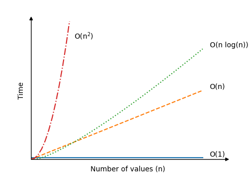
Here is how time increases when the number of values \(n\) increase for different algorithms:
Best, Average and Worst Case
'Worst case' time complexity has already been mentioned when explaining Big O notation, but how can an algorithm have a worst case scenario?
The algorithm that finds the lowest value in an array with \(n\) values requires \(n\) operations to do so, and that is always the same. So this algorithm has the same best, average, and worst case scenarios.
But for many other algorithms we will look at, if we keep the number of values \(n\) fixed, the runtime can still change a lot depending on the actual values.
Without going into all the details, we can understand that a sorting algorithm can have different runtimes, depending on the values it is sorting.
Just imagine you have to sort 20 values manually from lowest to highest:
8, 16, 19, 15, 2, 17, 4, 11, 6, 1, 7, 13, 5, 3, 9, 12, 14, 20, 18, 10
This will take you some seconds to finish.
Now, imagine you have to sort 20 values that are almost sorted already:
1, 2, 3, 4, 5, 20, 6, 7, 8, 9, 10, 11, 12, 13, 14, 15, 16, 17, 18, 19
You can sort the values really fast, by just moving 20 to the end of the list and you are done, right?
Algorithms work similarly: For the same amount of data they can sometimes be slow and sometimes fast. So to be able to compare different algorithms' time complexities, we usually look at the worst-case scenario using Big O notation.
Big O Explained Mathematically
Depending on your background in Mathematics, this section might be hard to understand. It is meant to create a more solid mathematical basis for those who need Big O explained more thoroughly.
If you do not understand this now, don't worry, you can come back later. And if the math here is way over your head, don't worry too much about it, you can still enjoy the different algorithms in this tutorial, learn how to program them, and understand how fast or slow they are.
In Mathematics, Big O notation is used to create an upper bound for a function, and in Computer Science, Big O notation is used to describe how the runtime of an algorithm increases when the number of data values \(n\) increase.
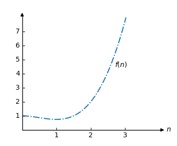
For example, consider the function:
\[f(n) = 0.5n^3 -0.75n^2+1 \]
The graph for the function \(f\) looks like this:
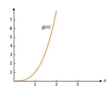
Consider another function:
\[g(n) = n^3 \]
Which we can draw like this:
Using Big O notation we can say that \(O(g(n))\) is an upper bound for \(f(n)\) because we can choose a constant \(C\) so that \(C \cdot g(n)>f(n)\) as long as \(n\) is big enough.
Ok, let's try. We choose \(C=0.75\) so that \(C \cdot g(n) = 0.75 \cdot n^3\).
Now let's draw \(0.75 \cdot g(n)\) and \(f(n)\) in the same plot:
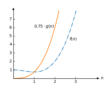
We can see that \(O(g(n))=O(n^3)\) is the upper bound for \(f(n)\) because \(0.75 \cdot g(n) > f(n)\) for all \(n\) larger than 1.
In the example above \(n\) must be larger than 1 for \(O(n^3)\) to be an upper bound. We call this limit \(n_0\).
Definition
Let \(f(n)\) and \(g(n)\) be two functions. We say that \(f(n)\) is \(O(g(n))\) if and only if there are positive constants \(C\) and \(n_0\) such that
\[ C \cdot g(n) > f(n) \]
for all \(n>n_0\).
When evaluating time complexity for an algorithm, it is ok that \(O()\) is only true for a large number of values \(n\), because that is when time complexity becomes important. To put it differently: if we are sorting, 10, 20 or 100 values, the time complexity for the algorithm is not so interesting, because the computer will sort the values in a short time anyway.

